Regression Analysis: Conceptual Foundations

Introduction

This tutorial introduces regression analysis — one of the most widely used statistical methods in linguistics, psychology, and the language sciences. Regression models allow us to assess whether and how predictor variables (independent variables) correlate with an outcome variable (dependent variable), while controlling for the effects of other predictors (Field, Miles, and Field 2012; Gries 2021; Winter 2019).

Tutorial Scope and Structure

This is Regression Analysis: Conceptual Foundations. It covers regression theory without R code.

Regression Analysis: Implementation in R (separate tutorial) shows how to run, diagnose, and report regressions using modern R packages.

Prerequisites:

• Basic Concepts in Quantitative Research
  
• Descriptive Statistics with R

What this tutorial covers:

1. What is regression and how does it work?
   
2. Types of regression models
   
3. Model assumptions and when they matter
   
4. Interpreting coefficients, p-values, and R²
   
5. Categorical predictors and interactions
   
6. Model fitting strategies
   
7. Sample size and power
   
8. Multicollinearity
   
9. Effect sizes
   
10. Reporting standards

What this does NOT cover:

• R implementation (see Part II)
  
• Mixed-effects models (see separate tutorial)
  
• Causal inference (regression ≠ causation)
  

---

Why Regression?

Regression models are popular because they:

1. Handle multiple predictors simultaneously — test the effect of one predictor while controlling for all others (multivariate analysis)
   
2. Are extremely flexible — can handle numeric, categorical, ordinal, and count outcomes
   
3. Produce interpretable output — coefficients, p-values, confidence intervals, effect sizes
   
4. Are conceptually accessible — mathematically simpler than many machine learning methods
   
5. Are widely reported — facilitates comparison across studies and meta-analysis

---

What Is Regression?

At its core, regression is a method for modeling the relationship between:

• One or more predictor variables (independent variables, IVs, explanatory variables)
  
• A single outcome variable (dependent variable, DV, response variable)

The fundamental regression equation is:

\[\text{Outcome} = \text{Intercept} + \text{Coefficient} \times \text{Predictor} + \text{Error}\]

Or in standard notation:

\[y = \alpha + \beta x + \epsilon\]

Where:

• \(y\) = the outcome we want to predict
  
• \(\alpha\) (alpha) = intercept — the predicted value of \(y\) when all predictors = 0
  
• \(\beta\) (beta) = coefficient (slope) — how much \(y\) changes for a 1-unit increase in \(x\)
  
• \(x\) = predictor variable
  
• \(\epsilon\) (epsilon) = residual (error) — the difference between observed and predicted \(y\)

A Concrete Example

Suppose we want to predict weight (kg) from height (cm). The regression equation might be:

\[\text{Weight} = -93.77 + 0.98 \times \text{Height}\]

Interpretation:

• Intercept (−93.77): A person with height = 0 cm would weigh −93.77 kg. (Nonsensical! This is why centering predictors matters — more later.)
  
• Coefficient (0.98): For every 1 cm increase in height, weight increases by 0.98 kg on average.
  
• Prediction: A person who is 180 cm tall is predicted to weigh: \(-93.77 + 0.98 \times 180 = 82.63\) kg.

The residual for this person is the difference between their actual weight and the predicted 82.63 kg.

---

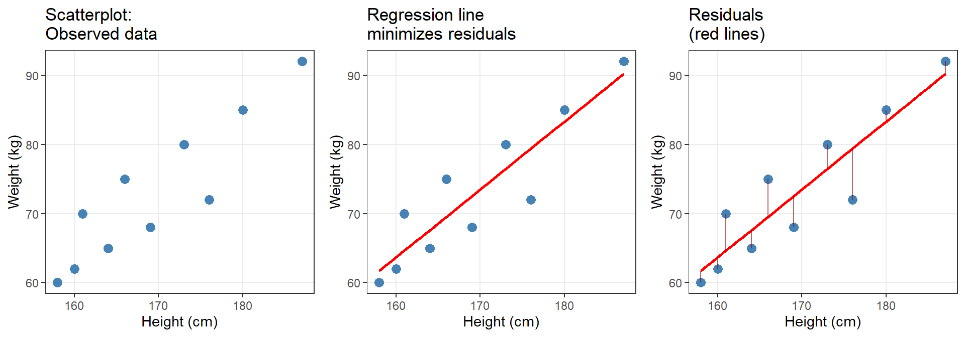
The Geometry of Regression: Finding the Best Line

Regression aims to find the line of best fit — the line that minimizes the sum of squared residuals (the vertical distances between observed data points and the regression line). This is called ordinary least squares (OLS) regression.

Key insight: The regression line is positioned such that the sum of squared residuals is minimized. No other line through the data would have a smaller total squared error.

---

Types of Regression Models

The type of regression you use depends on the measurement scale of your outcome variable:

Outcome variable type	Regression type	Example
Continuous (numeric), normally distributed, no extreme outliers	Simple/Multiple Linear Regression	Predicting reaction time (ms) from word frequency
Binary (two categories: yes/no, success/failure)	Logistic Regression	Predicting whether a speaker uses -er vs. more
Ordinal (ordered categories, e.g., Likert scale: strongly disagree → strongly agree)	Ordinal Regression	Predicting acceptability ratings (1–7 scale)
Count (non-negative integers: 0, 1, 2, …) of rare events	Poisson Regression	Predicting number of discourse particles per utterance
Continuous with outliers that cannot be removed	Robust Regression	Predicting word frequency with extreme high-frequency function words

Fixed-Effects vs. Mixed-Effects Regression

Fixed-effects regression (this tutorial) assumes:

• All data points are independent
  
• No hierarchical structure (no nesting: e.g., students within classes, words within speakers)

Mixed-effects regression (separate tutorial) is required when:

• Data points are nested or grouped (e.g., multiple observations per participant)
  
• You need random effects to model subject/item variability

If your data has repeated measures or hierarchical structure, see the mixed-effects tutorial.

---

Model Assumptions

Regression models rest on mathematical assumptions. Violating these assumptions can produce unreliable results.

Assumptions for Linear Regression

1. Linearity: The relationship between predictors and outcome is linear
   
2. Independence: Observations are independent (no autocorrelation, no nesting)
   
3. Homoscedasticity: Residuals have constant variance across all levels of predictors
   
4. Normality of residuals: Residuals are approximately normally distributed
   
5. No perfect multicollinearity: Predictors are not perfectly correlated with each other
   
6. No influential outliers: Extreme data points do not dominate the model fit

When assumptions are violated:

Violation	Solution
Non-linearity	Transform variables (log, sqrt) or use non-linear models
Non-independence	Use mixed-effects models or account for clustering
Heteroscedasticity	Use robust standard errors or transform outcome
Non-normal residuals	For large samples (n > 30–50), Central Limit Theorem provides protection; otherwise transform or use non-parametric methods
Multicollinearity	Remove redundant predictors or use regularization
Outliers	Use robust regression or remove outliers with strong justification

Assumptions for Logistic/Ordinal/Poisson Regression

Non-linear regressions (logistic, ordinal, Poisson) do not assume:

• Normality of the outcome
  
• Homoscedasticity

But they do assume:

• Independence of observations
  
• No multicollinearity among predictors
  
• Linearity of the logit (for logistic regression: the log-odds are linear in the predictors)
  
• No complete separation (for logistic: if a predictor perfectly predicts the outcome, the model breaks)

---

Interpreting Regression Output

A regression model produces several key statistics. Here’s what they mean:

Coefficients (β)

Interpretation depends on regression type:

Regression type	Coefficient interpretation
Linear	A 1-unit increase in \(x\) is associated with a \(\beta\)-unit change in \(y\)
Logistic	A 1-unit increase in \(x\) multiplies the odds of the outcome by \(e^\beta\)
Ordinal	A 1-unit increase in \(x\) changes the log-odds of being in a higher category by \(\beta\)
Poisson	A 1-unit increase in \(x\) multiplies the expected count by \(e^\beta\)

Standard Error (SE)

The SE tells us how much the coefficient would vary if we repeated the study many times with different samples from the same population. Smaller SE = more precise estimate.

\[\text{SE} = \frac{SD}{\sqrt{n}}\]

t-value (linear) or z-value (logistic/Poisson)

\[t = \frac{\text{Coefficient}}{\text{SE}}\]

The t- or z-value measures how many standard errors the coefficient is away from zero. Larger absolute values → stronger evidence against H₀: β = 0.

p-value

The probability of observing a coefficient this large (or larger) if the true effect were zero. p < .05 is the conventional threshold for “statistical significance.”

p-values ≠ Effect Size

A tiny, practically meaningless effect can be “significant” with a large enough sample. A large, important effect can be “non-significant” with a small sample. Always report effect sizes alongside p-values.

R² (for linear regression)

R² = proportion of variance in the outcome explained by the model.

• R² = 0: Model explains no variance (useless)
  
• R² = 0.10: 10% of variance explained (weak but possibly meaningful in social sciences)
  
• R² = 0.50: 50% of variance explained (strong)
  
• R² = 1: Perfect fit (only possible with measurement error = 0)

Adjusted R² penalizes models for including many predictors. It is always ≤ R² and prevents overfitting.

\[R^2_{\text{adjusted}} = 1 - \frac{(1 - R^2)(n - 1)}{n - k - 1}\]

where k = number of predictors.

AIC and BIC (model comparison)

Akaike Information Criterion (AIC) and Bayesian Information Criterion (BIC) balance model fit against complexity. Lower values = better models.

\[\text{AIC} = -2 \times \text{LogLikelihood} + 2k\]

\[\text{BIC} = -2 \times \text{LogLikelihood} + k \times \log(n)\]

Use AIC/BIC to compare models fit on the same data:

• ΔAIC < 2: Models are essentially equivalent
  
• ΔAIC = 2–7: Moderate evidence for the model with lower AIC
  
• ΔAIC > 10: Strong evidence for the model with lower AIC

---

Exercises: Regression Basics

Q1. What does the intercept (α) in a regression represent?

The slope of the regression line
The strength of the correlation between predictors and outcome
The predicted value of the outcome when all predictors equal zero
The p-value of the model

---

Q2. A logistic regression reports a coefficient β = 0.693 for a predictor. What is the odds ratio (OR)?

OR = 1.693 (= 1 + β)
OR = 0.693 (same as β)
OR = 0.5 (= 1/2)
OR = 2.0 (= e^0.693)

---

Q3. Which regression assumption is VIOLATED if residuals increase in variance as the predicted values increase (forming a funnel shape in a residuals plot)?

Normality of residuals
Independence of observations
Linearity
Homoscedasticity (constant variance of residuals)

---

Q4. A researcher reports: ‘Our model explains 45% of the variance (R² = 0.45).’ What does this mean?

45% of the variability in the outcome is accounted for by the predictors in the model
There is a 45% probability that the model is correct
The model makes correct predictions 45% of the time
45% of the data points fall exactly on the regression line

---

Categorical Predictors in Regression

So far we have discussed regression with continuous predictors (e.g., year, height, test scores). But regression can also handle categorical predictors (e.g., gender, experimental condition, language variety).

When a categorical predictor enters a regression, R automatically converts it into dummy variables (also called indicator variables or contrast coding).

How Dummy Coding Works

Suppose we have a predictor Group with three levels: A, B, C. R creates dummy variables:

Group	Dummy_B	Dummy_C
A	0	0
B	1	0
C	0	1

The regression equation becomes:

\[y = \alpha + \beta_1 \times \text{Dummy\_B} + \beta_2 \times \text{Dummy\_C} + \epsilon\]

Interpretation:

• α (Intercept): Mean of the reference group (Group A)
  
• β₁: Difference between Group B and Group A
  
• β₂: Difference between Group C and Group A

Changing the Reference Level

By default, R uses alphabetical ordering to determine the reference level. You can change this with:

data$Group <- relevel(data$Group, ref = "B")  # Set B as reference  

Always check which level is the reference when interpreting categorical predictors!

Example: Gender as a Predictor

If Gender has levels “Female” and “Male” (alphabetically, Female is first):

\[\text{Outcome} = \alpha + \beta \times \text{Male}\]

Where:

• α = mean outcome for females (reference group)
  
• β = difference between males and females (Male mean − Female mean)

If β = 15 and p < .05, males score 15 points higher on average than females.

---

Exercises: Categorical Predictors

Q1. A regression with predictor Condition (3 levels: A, B, C) produces two dummy variables: Condition_B and Condition_C. What is the reference level?

B (the first dummy variable)
C (the last dummy variable)
A (the level not represented by a dummy variable)
There is no reference level — all are equally represented

---

Q2. In a model with Gender (Female, Male) as a predictor, the intercept = 50 and the coefficient for Male = −10. What is the predicted outcome for females?

50 (the intercept = mean of the reference group)
40 (= 50 − 10)
Cannot be determined without more information
60 (= 50 + 10)

---

Interactions in Regression

An interaction occurs when the effect of one predictor depends on the level of another predictor. Interactions are non-additive effects.

Additive vs. Interactive Effects

Additive model (no interaction):

\[y = \alpha + \beta_1 x_1 + \beta_2 x_2\]

The effect of \(x_1\) is the same regardless of \(x_2\).

Interactive model:

\[y = \alpha + \beta_1 x_1 + \beta_2 x_2 + \beta_3 (x_1 \times x_2)\]

The effect of \(x_1\) changes depending on the value of \(x_2\).

Example: Teaching Method × Prior Knowledge

Imagine:

• Predictor 1: Teaching method (traditional vs. innovative)
  
• Predictor 2: Prior knowledge (low vs. high)
  
• Outcome: Test score

Additive model predicts:

• Innovative method adds 10 points for everyone
  
• High prior knowledge adds 15 points for everyone
  
• A high-knowledge student in the innovative method scores: baseline + 10 + 15 = 25 points above baseline

Interactive model might find:

• Innovative method helps low-knowledge students (+15 points) but not high-knowledge students (+2 points)
  
• This is an interaction: the effect of teaching method depends on prior knowledge

In regression output, the interaction coefficient tests: “Is the effect of \(x_1\) significantly different across levels of \(x_2\)?”

---

Exercises: Interactions

Q1. In a model with interaction A × B, predictor A is non-significant but the interaction is significant. Should you remove predictor A from the model?

No — you must retain both main effects if their interaction is included
Yes — non-significant predictors should always be removed
Yes — the interaction fully explains the effect of A
It depends on the AIC value

---

Q2. A significant interaction between Condition (2 levels) and Gender (2 levels) means:

Males and females differ in the outcome variable
The model explains more than 50% of the variance
Both Condition and Gender have significant main effects
The effect of Condition is different for males vs. females (or vice versa)

---

Model Fitting and Selection

Model fitting (also called model selection) is the process of deciding which predictors to include in the final model. The goal: find a model that explains the data well without including unnecessary predictors.

The Principle of Parsimony

Occam’s Razor: Among competing models, prefer the simplest one that explains the data adequately. Including too many predictors:

• Increases the risk of overfitting (the model fits the sample but not the population)
  
• Makes interpretation harder
  
• Reduces statistical power

Model Fitting Strategies

1. Theory-driven (recommended): Include predictors based on theory and prior research. Test the full theoretically motivated model.

2. Stepwise procedures (use with caution):

   • Forward selection: Start with no predictors; add predictors one at a time based on improvement in fit
     
   • Backward elimination: Start with all predictors; remove non-significant predictors one at a time
     
   • Automated stepwise: Algorithm adds/removes predictors based on AIC or BIC

Problems with Automated Stepwise Selection

Automated stepwise procedures are convenient but problematic:

• High risk of overfitting
  
• Capitalize on chance (spurious correlations)
  
• Ignore theoretical considerations
  
• p-values and confidence intervals are no longer trustworthy
  
• Different orderings of predictors can yield different “final” models

Best practice: Use theory to guide model specification. If you must use stepwise, treat it as exploratory and validate findings in an independent dataset.

Comparing Models: Nested Model Comparison

To test whether a predictor (or set of predictors) significantly improves the model:

1. Fit a full model with the predictor(s)
   
2. Fit a reduced model without the predictor(s)
   
3. Use ANOVA (for linear models) or likelihood ratio test (for GLMs) to compare

If the full model significantly outperforms the reduced model, retain the predictor.

---

Exercises: Model Fitting

Q1. A researcher reports: ‘We used automated stepwise regression (backward elimination) and retained predictors with p < .05.’ What is the main problem with this approach?

Backward elimination should start with no predictors, not all predictors
Stepwise regression is the gold standard and has no problems
p < .05 is too strict — should use p < .10 for model selection
Stepwise procedures capitalize on chance, inflate Type I error, and ignore theory

---

Q2. You compare two nested models using ANOVA. Model 1 has 3 predictors (R² = 0.25); Model 2 has 5 predictors (R² = 0.27). The ANOVA p-value is .18. What should you conclude?

Retain Model 2 — it has higher R²
p > .05 means neither model is significant
Both models are equally good — use either one
Retain Model 1 (the simpler model) — the additional predictors do not significantly improve fit

---

Sample Size and Statistical Power

How Much Data Do You Need?

Following Green (1991) and Field, Miles, and Field (2012), here are rules of thumb for linear regression:

Let k = number of predictors (for categorical predictors with > 2 levels, count each dummy variable).

• For overall model fit (R²): \(n \geq 50 + 8k\)
  
• For testing individual predictors: \(n \geq 104 + k\)
  
• If interested in both: Use the larger value

Example: A model with 5 predictors testing both overall fit and individual coefficients requires:

\[n \geq \max(50 + 8 \times 5, 104 + 5) = \max(90, 109) = 109\]

You need at least 109 observations.

Why These Rules?

These are based on achieving 80% statistical power to detect medium-sized effects (Cohen’s f² = 0.15) at α = .05.

If your expected effects are smaller, you need more data. If effects are larger, you might get away with less — but it’s safer to err on the side of larger samples.

What If Your Sample Is Too Small?

Options:

1. Collect more data (ideal but often impractical)
   
2. Reduce the number of predictors (test only the most important ones)
   
3. Report the analysis as exploratory and note the limited power
   
4. Conduct a power analysis to estimate your actual statistical power given your sample size

---

Exercises: Sample Size

Q1. You fit a model with 8 predictors and n = 75. According to Green’s (1991) rule, is your sample size adequate for testing individual predictors?

No — you need n ≥ 104 + 8 = 112
Yes — 75 observations is always sufficient
Yes — n > 50 + 8k = 114
No — you need at least 200 observations for any regression

---

Q2. A colleague says: ‘I have 200 participants, which is plenty for any regression.’ Is this correct?

No — you always need at least 500 participants
Yes — as long as you use stepwise selection
Not necessarily — it depends on the number of predictors and expected effect size
Yes — 200 is always sufficient for regression

---

Multicollinearity

Multicollinearity occurs when predictors in a regression model are highly correlated with each other. This is a problem because it inflates standard errors and makes coefficients unstable.

Why Is Multicollinearity a Problem?

When two predictors are highly correlated:

• They share variance in explaining the outcome
  
• The model cannot distinguish their unique contributions
  
• Coefficients become unreliable: small changes in the data produce large changes in estimates
  
• Standard errors inflate → p-values become untrustworthy

Example: If you include both “height in cm” and “height in inches” as predictors, they are perfectly collinear. The model cannot tell which is “responsible” for predicting the outcome.

Detecting Multicollinearity: VIF

The Variance Inflation Factor (VIF) quantifies how much the variance of a coefficient is inflated due to collinearity.

\[\text{VIF} = \frac{1}{1 - R^2_j}\]

where \(R^2_j\) is the R² from a regression predicting predictor \(j\) from all other predictors.

Interpretation:

VIF value	Interpretation	Action
VIF = 1	No collinearity	✓ No problem
VIF < 3	Low collinearity	✓ Acceptable
VIF = 3–5	Moderate collinearity	⚠ Concerning
VIF = 5–10	High collinearity	⚠ Problematic — consider removing
VIF > 10	Severe collinearity	✗ Remove predictor

Mean VIF: The average VIF across all predictors should be close to 1. A mean VIF >> 1 suggests overall collinearity issues.

Solutions to Multicollinearity

1. Remove one of the correlated predictors (keep the most theoretically important one)
   
2. Combine correlated predictors into a single composite variable (e.g., via PCA or averaging)
   
3. Center predictors (reduces collinearity in models with interactions)
   
4. Collect more data (in some cases, collinearity is a sample-specific artifact)

When Multicollinearity Doesn’t Matter

If your goal is prediction (not interpretation), multicollinearity is less problematic. You care about accurate predictions, not about which predictor is “responsible.”

Multicollinearity is a serious issue only when you want to interpret individual coefficients.

---

Exercises: Multicollinearity

Q1. A model includes predictors A, B, and C. Predictor B has VIF = 8.5. What should you do?

Remove predictors A and C instead
Transform predictor B to reduce VIF
Consider removing predictor B, as VIF > 5 indicates problematic multicollinearity
Nothing — VIF < 10 is always acceptable

---

Q2. Why does multicollinearity inflate standard errors?

Collinear predictors cancel each other out mathematically
The sample size effectively decreases when predictors are correlated
Multicollinearity violates the independence assumption
The model cannot distinguish which predictor is responsible for the shared variance, creating uncertainty

---

Effect Sizes for Regression

Cohen’s f² for Linear Regression

Cohen’s f² measures the unique contribution of a predictor (or set of predictors) to R²:

\[f^2 = \frac{R^2_{\text{full}} - R^2_{\text{reduced}}}{1 - R^2_{\text{full}}}\]

f² value	Interpretation
0.02	Small effect
0.15	Medium effect
0.35	Large effect

Odds Ratios (OR) for Logistic Regression

For logistic regression, exponentiated coefficients = odds ratios:

\[\text{OR} = e^\beta\]

OR value	Interpretation
OR = 1	No effect (predictor does not change odds)
OR = 1.5	Small effect (50% increase in odds)
OR = 2	Predictor doubles the odds
OR = 3	Medium effect (200% increase in odds)
OR = 0.5	Predictor halves the odds
OR < 1	Negative effect (decreases odds)
OR > 1	Positive effect (increases odds)

Incidence Rate Ratios (IRR) for Poisson Regression

For Poisson regression, exponentiated coefficients = incidence rate ratios:

\[\text{IRR} = e^\beta\]

Interpretation is identical to odds ratios, but applied to expected counts rather than odds.

---

Exercises: Effect Sizes

Q1. A linear regression adds 3 predictors to a baseline model. R²_baseline = 0.10, R²_full = 0.25. What is Cohen’s f² for the added predictors?

f² = 0.20 (= (0.25 − 0.10) / (1 − 0.25)) — a medium effect
f² = 0.15 (= 0.25 − 0.10)
f² = 0.35 (a large effect)
Cannot be calculated without knowing n

---

Q2. A logistic regression reports β = −0.511 for predictor X. What is the odds ratio, and how do you interpret it?

OR = −0.511 (same as β)
OR = 0.40 (= 1 − 0.60) — predictor X reduces the odds to 40%
OR = 0.60 (= e^−0.511) — predictor X reduces the odds by 40%
OR = 1.67 (= 1 / 0.60) — predictor X increases the odds by 67%

---

Reporting Regression Results

What to Include in a Regression Report

A complete regression analysis report includes:

1. Model specification: Which predictors were included and why
   
2. Sample size: Total n and n per group (if categorical predictors)
   
3. Model diagnostics: Statement that assumptions were checked (and how)
   
4. Overall model fit: F-statistic (linear) or χ² (GLM), p-value, R² (linear) or pseudo-R² (GLM)
   
5. Coefficients table: β, SE, t/z, p, 95% CI for each predictor
   
6. Effect sizes: Cohen’s f² (linear), odds ratios (logistic), etc.
   
7. Interpretation: What do the significant predictors mean in practical terms?

APA-Style Regression Table

A well-formatted table should include:

Predictor	B	SE	95% CI	β (std.)	t	p
Intercept	50.23	2.14	[46.02, 54.44]	—	23.47	< .001
Age	1.45	0.32	[0.82, 2.08]	0.28	4.53	< .001
Gender (Male)	−5.12	1.87	[−8.79, −1.45]	−0.17	−2.74	.006

Caption: Regression coefficients predicting test scores. Standardized coefficients (β) are provided for continuous predictors. Gender reference level: Female. n = 200, R² = .18, F(2, 197) = 21.6, p < .001.

Example Write-Up

A multiple linear regression was conducted to predict test scores from age and gender (n = 200). Diagnostic plots indicated that model assumptions were met. The overall model was significant, F(2, 197) = 21.6, p < .001, and explained 18% of the variance in test scores (R² = .18, adjusted R² = .17). Age was a significant positive predictor (β = 1.45, SE = 0.32, 95% CI [0.82, 2.08], t = 4.53, p < .001, β_std = 0.28): each additional year of age was associated with a 1.45-point increase in test scores. Gender was also significant (β = −5.12, SE = 1.87, 95% CI [−8.79, −1.45], t = −2.74, p = .006, β_std = −0.17): males scored 5.12 points lower than females on average. Effect sizes were small to moderate (Cohen’s f² = 0.22).

---

Quick Reference

Choosing the Right Regression Model

Outcome variable	Regression type	Key assumptions
Continuous, normal, no outliers	Linear	Linearity, independence, homoscedasticity, normality of residuals
Binary (2 categories)	Logistic	Independence, linearity of logit, no complete separation
Ordinal (ordered categories)	Ordinal	Independence, proportional odds
Count (rare events)	Poisson	Independence, mean = variance
Continuous with outliers	Robust	Same as linear, but robust to outliers

---

Model Diagnostics Checklist

Diagnostic	What to look for
Overall model quality	All diagnostic panels acceptable
Linearity	Residuals vs. Fitted: random scatter (no pattern)
Homoscedasticity	Scale-Location: horizontal line (no funnel)
Normality of residuals	Q-Q plot: points on diagonal line
Outliers	Cook’s distance: no points beyond threshold
Multicollinearity	VIF < 3 (ideally); < 5 (acceptable); < 10 (maximum)
Independence	Durbin-Watson test: p > .05 (no autocorrelation)

---

Effect Size Guidelines

Linear regression (Cohen’s f²):

f²	Interpretation
0.02	Small
0.15	Medium
0.35	Large

Logistic regression (Odds Ratio):

OR	Interpretation
OR = 1	No effect
OR = 1.5	Small effect (50% increase in odds)
OR = 3.0	Medium effect (200% increase in odds)
OR = 6.0	Large effect (500% increase in odds)

---

Sample Size Requirements

Following Green (1991), for medium effect sizes (80% power, α = .05):

Goal	Minimum n
Testing overall model	50 + 8k
Testing individual predictors	104 + k
Both	Take the larger value

where k = number of predictors (count each dummy variable separately).

---

Common Mistakes to Avoid

1. Ignoring assumptions — Always check diagnostics before interpreting results
   
2. Treating p < .05 as proof — Statistical significance ≠ practical importance
   
3. Not reporting effect sizes — Coefficients alone are insufficient
   
4. Using automated stepwise selection uncritically — Theory should guide model building
   
5. Removing the intercept without justification — The intercept is almost always needed
   
6. Not centering continuous predictors in interaction models — Leads to multicollinearity
   
7. Confusing correlation with causation — Regression shows association, not causation
   
8. Not checking for multicollinearity — Can silently invalidate results
   
9. Overfitting — Including too many predictors for the sample size
   
10. Not validating findings — Replication in independent data is essential

---

Citation & Session Info

Schweinberger, Martin. 2026. Regression Analysis: Conceptual Foundations. Brisbane: The University of Queensland. url: https://ladal.edu.au/tutorials/regression_concepts/regression_concepts.html (Version 2026.02.16).

@manual{schweinberger2026regression_concepts,  
  author = {Schweinberger, Martin},  
  title = {Regression Analysis: Conceptual Foundations},  
  note = {https://ladal.edu.au/tutorials/regression_concepts/regression_concepts.html},  
  year = {2026},  
  organization = {The University of Queensland, Australia. School of Languages and Cultures},  
  address = {Brisbane},  
  edition = {2026.02.16}  
}  

sessionInfo()  

R version 4.4.2 (2024-10-31 ucrt)
Platform: x86_64-w64-mingw32/x64
Running under: Windows 11 x64 (build 26200)

Matrix products: default


locale:
[1] LC_COLLATE=English_United States.utf8 
[2] LC_CTYPE=English_United States.utf8   
[3] LC_MONETARY=English_United States.utf8
[4] LC_NUMERIC=C                          
[5] LC_TIME=English_United States.utf8    

time zone: Australia/Brisbane
tzcode source: internal

attached base packages:
[1] stats     graphics  grDevices datasets  utils     methods   base     

other attached packages:
 [1] cowplot_1.2.0    lubridate_1.9.4  forcats_1.0.0    stringr_1.5.1   
 [5] dplyr_1.2.0      purrr_1.0.4      readr_2.1.5      tidyr_1.3.2     
 [9] tibble_3.2.1     ggplot2_4.0.2    tidyverse_2.0.0  checkdown_0.0.13

loaded via a namespace (and not attached):
 [1] generics_0.1.3     renv_1.1.1         stringi_1.8.4      lattice_0.22-6    
 [5] hms_1.1.3          digest_0.6.39      magrittr_2.0.3     evaluate_1.0.3    
 [9] grid_4.4.2         timechange_0.3.0   RColorBrewer_1.1-3 fastmap_1.2.0     
[13] jsonlite_1.9.0     Matrix_1.7-2       mgcv_1.9-1         scales_1.4.0      
[17] codetools_0.2-20   cli_3.6.4          rlang_1.1.7        litedown_0.9      
[21] commonmark_2.0.0   splines_4.4.2      withr_3.0.2        yaml_2.3.10       
[25] tools_4.4.2        tzdb_0.4.0         vctrs_0.7.1        R6_2.6.1          
[29] lifecycle_1.0.5    htmlwidgets_1.6.4  pkgconfig_2.0.3    pillar_1.10.1     
[33] gtable_0.3.6       glue_1.8.0         xfun_0.56          tidyselect_1.2.1  
[37] rstudioapi_0.17.1  knitr_1.51         farver_2.1.2       htmltools_0.5.9   
[41] nlme_3.1-166       rmarkdown_2.30     labeling_0.4.3     compiler_4.4.2    
[45] S7_0.2.1           markdown_2.0      

---

Back to top

Back to HOME

---

References

Field, Andy, Jeremy Miles, and Zoe Field. 2012. Discovering Statistics Using r. Vol. 50. Sage. https://doi.org/https://doi.org/10.5860/choice.50-2114.

Green, Samuel B. 1991. “How Many Subjects Does It Take to Do a Regression Analysis.” Multivariate Behavioral Research 26 (3): 499–510. https://doi.org/https://doi.org/10.1207/s15327906mbr2603_7.

Gries, Stefan Th. 2021. Statistics for Linguistics Using r: A Practical Introduction. Berlin & New York: Mouton de Gruyter.

Winter, Bodo. 2019. Statistics for Linguists: An Introduction Using r. Routledge. https://doi.org/https://doi.org/10.4324/9781315165547.

References

Field, Andy, Jeremy Miles, and Zoë Field. 2012. Discovering Statistics Using r. London: SAGE Publications.